The -0.35 Illusion: What Your Backtest Doesn't Know About Correlation

Part 67 is the first of a 3-part series on correlations

This is part 67 of my series — Building & Scaling Algorithmic Trading Strategies

---

The V6 Dual Allocator uses TLT as a hedge. The logic is simple: stocks and bonds are negatively correlated, so when SPY drops, TLT should rise. This reduces portfolio volatility and cushions drawdowns.

Except when it doesn’t.

In 2022, SPY fell 18%. TLT fell 31%. The hedge didn’t hedge — it actually amplified.

This isn’t a bug in my strategy. It’s a fundamental problem with how we think about correlation. The number we compute from historical data — call it ρ — is not the number that governs the next crisis.

This series will explore why correlations break, how to model regime-dependent relationships, and what we can actually do about it in live portfolios.

---

The Unconditional Lie

When you calculate correlation between SPY and TLT over a long period, you get something like -0.30 to -0.35. This is the unconditional correlation — the average relationship across all market conditions.

The problem is that “all market conditions” includes both calm periods (where you don’t need the hedge) and crisis periods (where you desperately do). And the correlation behaves very differently in each.

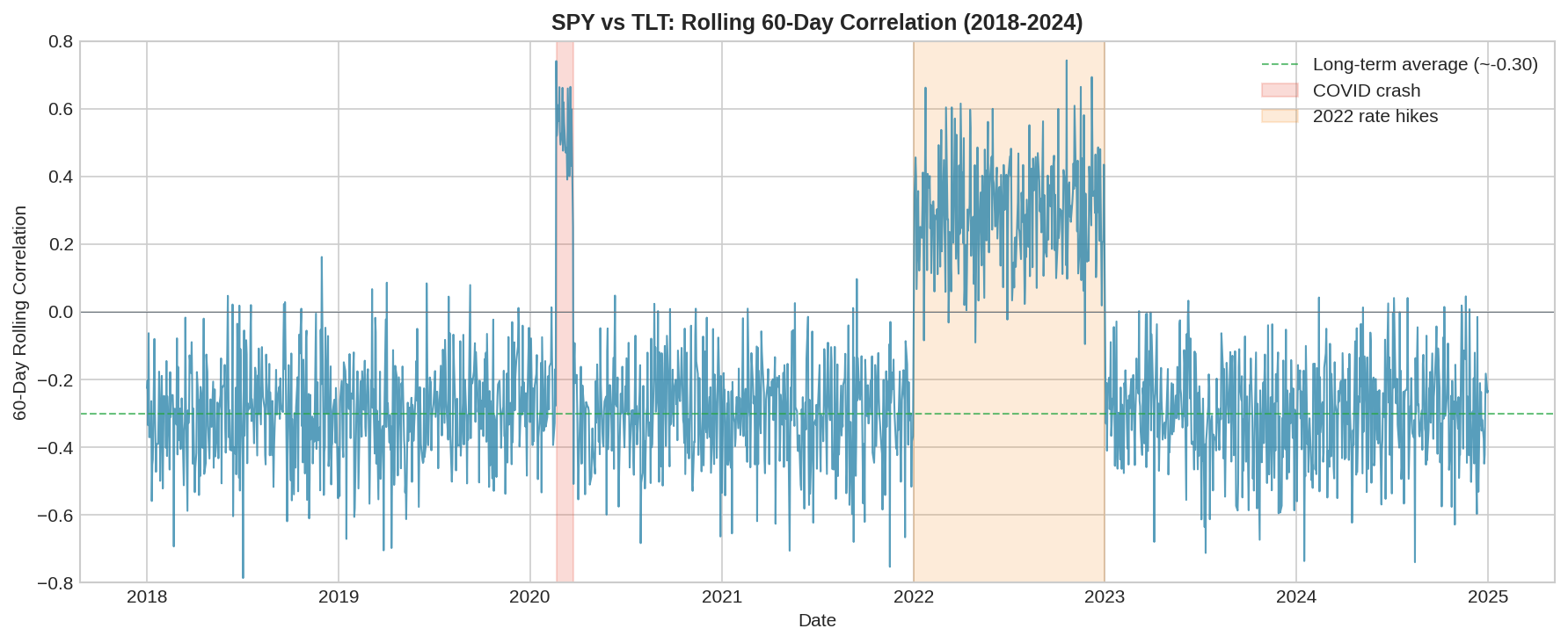
The chart above shows 60-day rolling correlation between SPY and TLT from 2018 to 2024. The long-term average hovers around -0.30, which looks great on paper. But look at what happens during the shaded periods:

March 2020 (COVID crash): Correlation spiked from -0.40 to +0.50 in about two weeks. Both stocks and bonds sold off simultaneously as investors liquidated everything for cash.

2022 (rate hikes): Correlation flipped positive for nearly the entire year, ranging from +0.20 to +0.50. This wasn’t a brief spike — it was a sustained regime change.

The unconditional correlation of -0.30 is a weighted average of two very different regimes: one where the hedge works (-0.40 to -0.50) and one where it doesn’t (+0.30 to +0.50). Using the average is like saying the average depth of a river is 3 feet when it’s 1 foot at the banks and 10 feet in the channel. You can still drown.

---

Conditional Correlation: The Real Relationship

The relationship between assets isn’t constant. It depends on the state of the market. This is conditional correlation.

A simple way to see this: bucket daily returns by magnitude and compute correlation within each bucket.

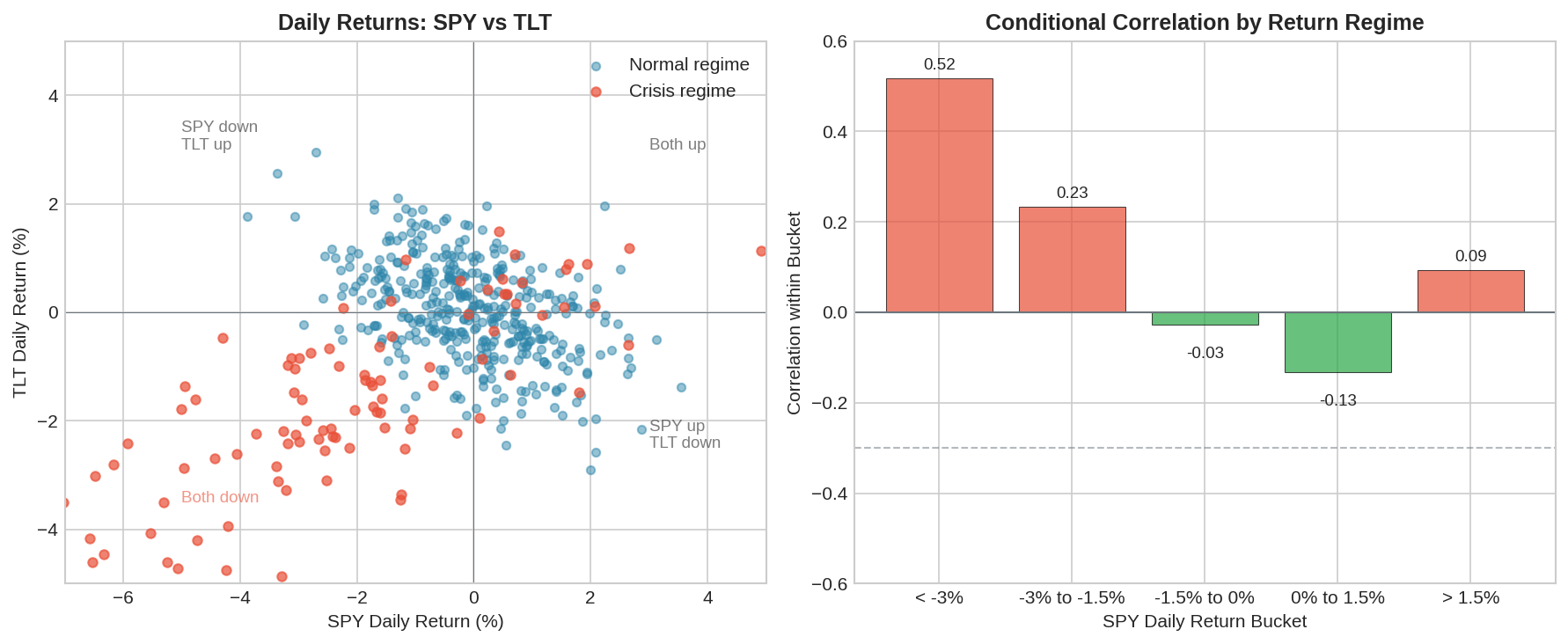
The left panel shows the scatter plot of daily SPY vs TLT returns. In normal conditions (blue dots), there’s a clear negative relationship — TLT tends to rise when SPY falls. But during crisis periods (red dots), both assets cluster in the lower-left quadrant. Both falling. Together.

The right panel quantifies this. When SPY is down more than 3% in a day, correlation with TLT is positive. The hedge becomes a second source of loss precisely when you need protection most.

This is the correlation paradox: the hedge correlation you compute from historical data understates the correlation you’ll experience in a crisis.

In chess, there’s a concept called “piece coordination” — the idea that your pieces should work together, reinforcing each other’s effectiveness. A knight and bishop covering complementary squares is powerful. But in crisis markets, your supposedly diversified assets stop coordinating. They become a king and rook both stuck behind the same pawn chain, useless when you need them.

---

The Math: Why This Happens

Correlation between two assets X and Y is defined as:

ρ(X,Y) = Cov(X,Y) / (σ_X × σ_Y)

Where:

• Cov(X,Y) = E[(X - μ_X)(Y - μ_Y)]

• σ_X and σ_Y are standard deviations

The key insight is that correlation depends on the joint distribution of returns. In normal times, SPY and TLT are driven by different factors: equity risk premium, duration risk, flight-to-quality flows. Their joint distribution looks roughly bivariate normal with negative correlation.

In a crisis, the driving factors change. Instead of fundamentals, you get:

1. Liquidity demand: Everyone sells everything to raise cash

2. Forced selling: Margin calls hit across asset classes

3. Contagion: Losses in one asset force sales in others

These factors affect both assets in the same direction. The joint distribution shifts — and so does correlation.

Let’s formalize this with a simple regime-switching model. Assume returns follow:

Normal regime (probability p):
  SPY ~ N(μ_S, σ_S)
  TLT ~ N(μ_T, σ_T)
  Correlation = ρ_normal ≈ -0.40

Crisis regime (probability 1-p):
  SPY ~ N(μ_S - δ_S, σ_S × k)   # Negative drift, higher vol
  TLT ~ N(μ_T - δ_T, σ_T × k)   # Also negative drift
  Correlation = ρ_crisis ≈ +0.40

If crises occur 15% of the time (p = 0.85), your unconditional correlation is roughly:

ρ_unconditional ≈ 0.85 × (-0.40) + 0.15 × (+0.40) = -0.28

That -0.28 looks fine in a backtest. But during the 15% of the time that matters — the crisis periods — you’re experiencing +0.40 correlation.

---

The Correlation Matrix Mirage

This problem compounds when you’re building multi-asset portfolios. Here’s what a typical correlation matrix looks like in calm vs. crisis conditions:

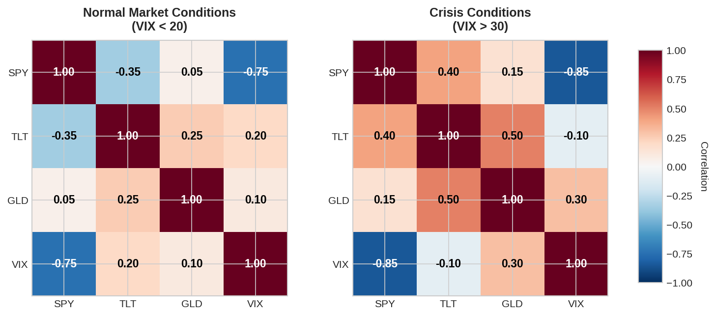
In normal conditions, you have genuine diversification. SPY and TLT are negatively correlated. Gold (GLD) is mostly uncorrelated with everything. VIX provides strong negative correlation to SPY (as expected).

In crisis conditions, correlations converge toward +1 for risky assets and the traditional relationships break down. TLT flips from -0.35 to +0.40 correlation with SPY. Even gold becomes more correlated with equities.

The technical term for this is correlation breakdown or correlation clustering. It’s well-documented in academic literature but consistently ignored in retail portfolio construction.

---

What This Means for the 60/40 Portfolio

The classic 60/40 portfolio (60% stocks, 40% bonds) is built on the assumption of stable negative correlation. The math looks great:

Portfolio variance = w_S² × σ_S² + w_T² × σ_T² + 2 × w_S × w_T × ρ × σ_S × σ_T

With ρ = -0.35:
  The cross term is negative
  Portfolio vol < weighted average of component vols
  Diversification "works"

With ρ = +0.40:
  The cross term is positive
  Portfolio vol > what you expected
  Diversification fails exactly when you need it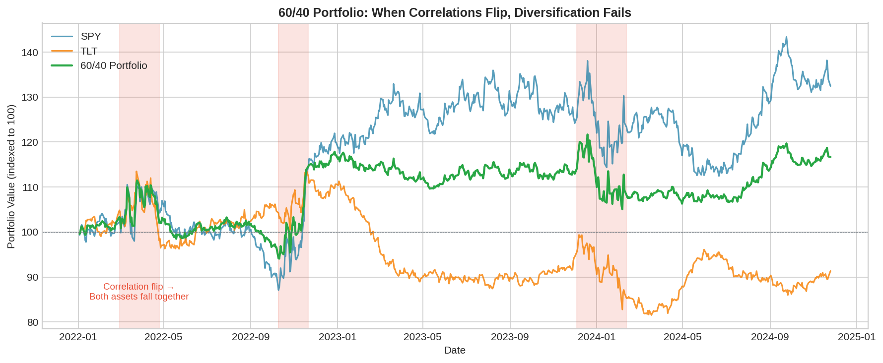

The shaded regions show periods where correlation flipped positive. Notice how the 60/40 portfolio (green line) fails to cushion the drawdowns. In fact, during these periods, the portfolio sometimes falls faster than SPY alone because TLT is adding to losses rather than offsetting them.

2022 was the worst year for 60/40 since 1937. Not because stocks fell — they’ve fallen worse before — but rather because bonds also fell simultaneously. The correlation assumption that underpins trillions of dollars in retirement assets simply didn’t hold.

---

Implications for V6 and Beyond

My V6 allocator uses TLT as a defensive position during negative momentum regimes. Based on the analysis above, this has a critical vulnerability: the TLT hedge may fail precisely during the fast, violent drawdowns where protection matters most.

Some immediate questions for Part 2 and 3:

1. Can we predict correlation regime changes? If correlation shifts are driven by volatility, VIX might be a leading indicator.

2. Are there better hedge instruments? Perhaps assets with more stable crisis behavior: cash, short-term treasuries, managed futures, or explicit tail hedges via options.

3. Should hedge sizing be dynamic? If we know correlation is unstable, maybe we should size hedges larger (assuming they might only be 50% effective) or add a second hedge layer.

4. What’s the cost of being wrong? Running the allocator with realistic correlation assumptions vs. the optimistic unconditional estimate.

---

The Chess Analogy

There’s a well-known chess principle: “The threat is stronger than the execution.” A piece threatening multiple squares controls the board more effectively than one committed to a single attack.

Correlation works the same way. A hedge that might work creates optionality — you have a piece that could go to multiple squares. But if you’ve sized your portfolio assuming the hedge will work with a specific correlation, you’ve committed the piece. When correlation flips, you’ve lost both the hedge benefit and the flexibility to adapt.

In Part 2, we’ll look at models that explicitly account for regime-dependent correlation: DCC-GARCH, copulas, and Hidden Markov approaches. The goal isn’t to predict crises (we can’t). It’s to build portfolios that don’t require stable correlation to survive.

---

Summary & Implications

• Unconditional correlation: The historical average across all regimes. Looks stable, but misleading.

• Conditional correlation: The correlation within specific market states. Changes dramatically in crises.

• Correlation breakdown: Correlations tend toward +1 during stress events. Diversification fails.

• 60/40 vulnerability Built on assumption of negative stock/bond correlation. 2022 showed the flaw.

Net-net, the overall implication for my Dual Allocator V6 is that TLT hedge may fail during fast drawdowns. So I need to build regime-aware sizing.

---

Coming up:

• Part 2: Dynamic Correlation Models — DCC-GARCH, copulas, and regime switching

• Part 3: Building Correlation-Aware Hedging — applying this to real portfolios

---

The analysis presented here is for educational purposes only and reflects my own portfolio construction challenges. Correlations discussed are illustrative; your own analysis may differ.

Past correlation behavior does not guarantee future behavior—that’s literally the point of this post.

---