
The Volatility Surface: Where Every Option Is a Different Bet on a Different Fear
Part 92 — The smile, the smirk, the term structure, and the four dimensions of vol surface trading

This is part 92 of my series — Building & Scaling Algorithmic Trading Strategies
Part 3 of the Synthetic Replication series. Part 1: Building blocks. Part 2: Replicating hedge fund strategies.
The Lie at the Heart of Options Pricing
Black-Scholes assumes one number — σ — describes the volatility of the underlying. Every option on the same stock, at every strike and every expiry, should use the same σ.
This has been empirically false since approximately October 19, 1987.
Before the ‘87 crash, the vol “smile” was roughly flat. After it, puts became permanently expensive relative to calls. The market learned that crashes happen, and it never forgot. That fear — that specific, priced-in fear of a left-tail event — is visible in every options chain you pull up today.
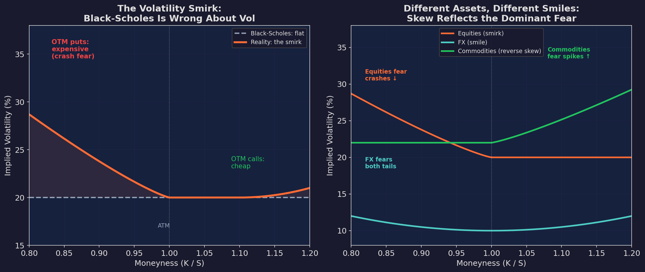
Left: Black-Scholes assumes flat vol (dashed gray). Reality is the smirk (orange) — OTM puts trade at significantly higher implied vol than ATM or OTM calls. That 8-10 vol point premium on the 20% OTM put is the market’s price for crash insurance. Right: different asset classes have different smile shapes. Equities smirk left (crash fear dominates). FX smiles symmetrically (both tails feared). Commodities skew right (spike fear dominates — no one worries about oil going to zero, they worry about it going to $200).
The shape of the smile tells you what the market is afraid of. And when the shape changes, it tells you the fear is shifting.
The Surface: Three Dimensions of Fear
The volatility smile is a 2D slice. The full picture is a surface — implied vol varies across both strike (moneyness) and time to expiry.
The vol surface for a typical equity index. The left-back corner (OTM puts, short-dated) is the most expensive — near-term crash protection commands the highest premium. The right-front corner (OTM calls, short-dated) is the cheapest. The surface flattens as you move to longer expirations — skew “decays” with time.
Two key features of the surface:
1. Skew is steeper for shorter expirations. A 7-day 90% moneyness put might trade at 35% IV while the same strike at 365 days trades at 24%. The short-dated put is more expensive per unit of time because short-dated crash fear is more acute — if a crash happens this week, you need protection now.
2. The surface is not static. After a selloff, the entire surface shifts up and steepens. After a long calm period, it shifts down and flattens. The surface is a living map of the market’s collective anxiety.
Term Structure: Near vs. Far
The second dimension of the surface — how IV varies with expiration at a fixed strike — is the term structure.
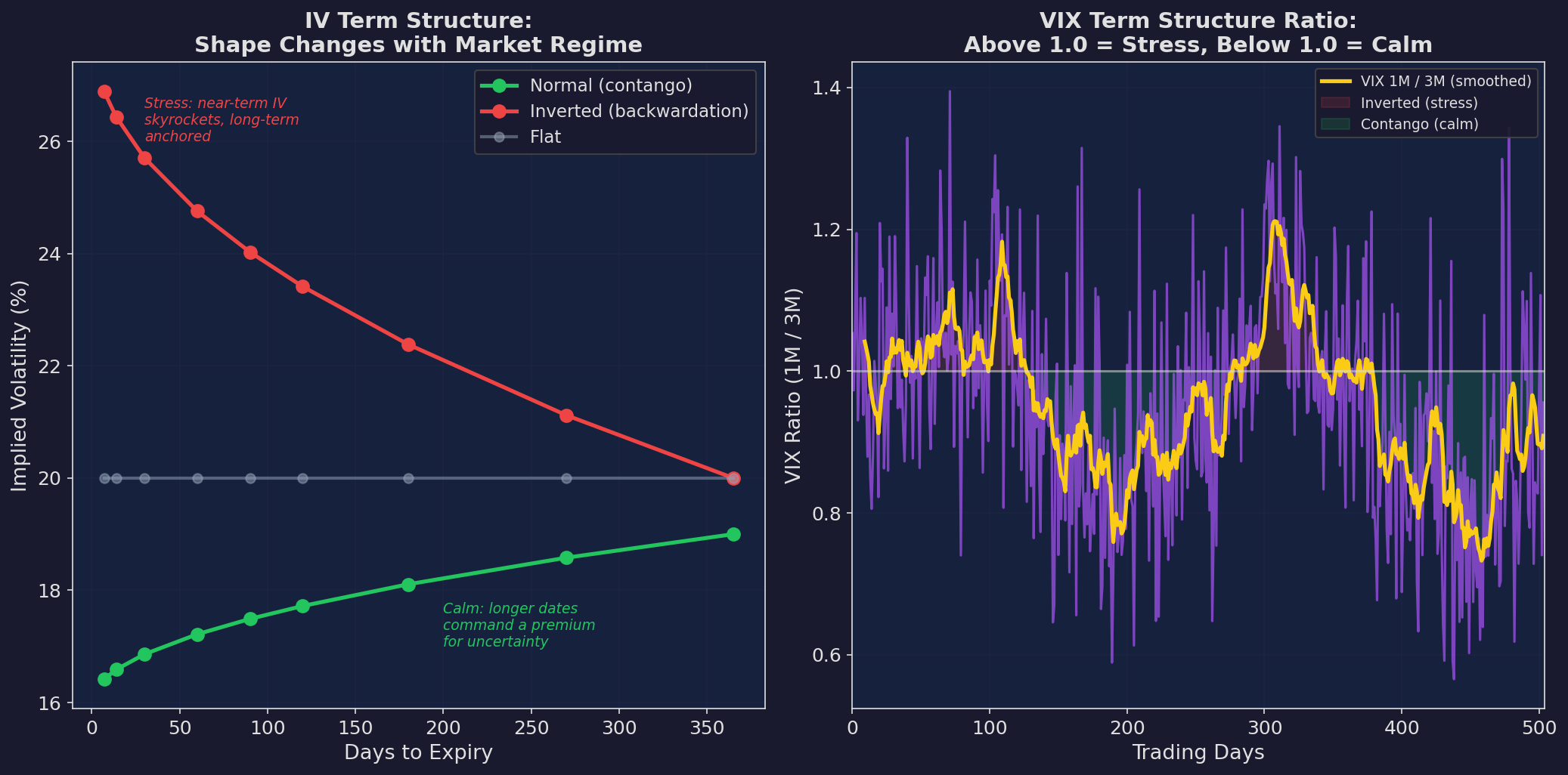
Left: three term structure shapes. Normal (contango, green): longer-dated options have higher IV because more uncertainty over longer horizons. Inverted (backwardation, red): near-term IV is elevated — a stress event is pricing into the front month. Flat (gray): no informational content. Right: the VIX term structure ratio (1-month VIX / 3-month VIX) over time. Above 1.0 = inverted = stress. Below 1.0 = contango = calm.
The term structure is a regime indicator, just like the VIX level itself. But it contains information that VIX alone misses:
VIX can be at 20 in both contango and backwardation. In contango (1M VIX = 20, 3M VIX = 22), the market expects the current level to persist — orderly uncertainty. In backwardation (1M VIX = 20, 3M VIX = 18), the market expects near-term stress to resolve — someone is paying up for immediate protection.
This links directly to the carry trade framework from Part 88: contango is “harvest” mode (sell near-term vol, it decays toward the lower long-term level). Backwardation is “retreat” mode (near-term vol is elevated for a reason).
Trading the Surface: Four Dimensions
Every vol surface trade targets one of four dimensions:
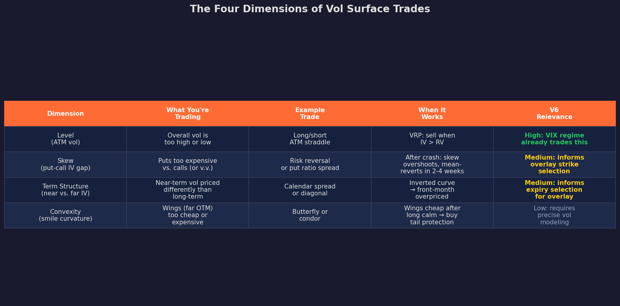
Let me unpack the two most tradeable dimensions.
Skew Trades: Selling Expensive Fear
Equity skew — the premium of OTM puts over OTM calls — is the most persistent and most tradeable feature of the vol surface.
The core trade: sell expensive put vol, buy cheap call vol. This is a risk reversal (Part 2), but now motivated by vol surface analysis rather than directional conviction.
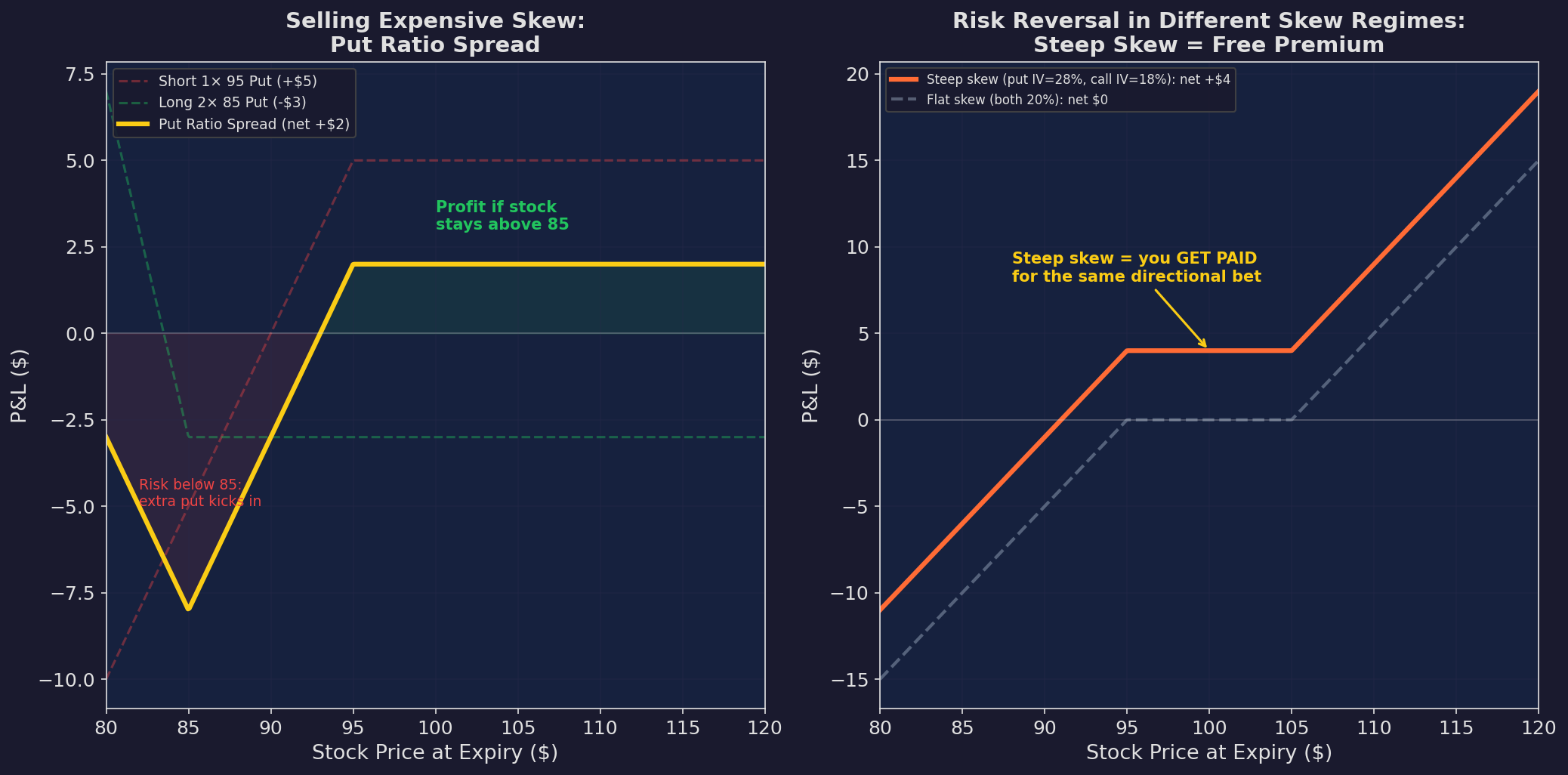
Left: the put ratio spread — sell one expensive near-ATM put, buy two cheaper far-OTM puts. You collect a net premium while maintaining downside protection below 85. Right: a risk reversal in two different skew regimes. When skew is steep (post-selloff), the short put is so expensive that you get PAID net premium for a bullish bet. When skew is flat, the same structure costs zero.
Why Steep Skew Is an Opportunity
After a selloff, skew overshoots. Put IV spikes to 30-35% while ATM vol is at 22% and call IV is at 18%. The 12-17 vol point skew is the market pricing in a continuation of the decline that is, on average, too pessimistic.
Research by Bollen and Whaley (2004) and Xing, Zhang, and Zhao (2010) documents that extreme skew predicts mean-reversion — steep skew is followed by declining skew as the panic premium dissipates. The half-life of a skew overshoot is approximately 2-4 weeks.
The Skew Mean-Reversion Signal
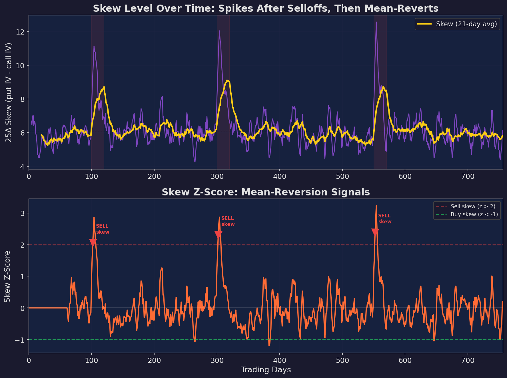
Top: 25-delta skew (put IV minus call IV) over time. It spikes during selloffs and mean-reverts within 2-4 weeks. Bottom: z-score of skew with trading thresholds. When skew z-score exceeds 2.0 (red markers), selling skew via risk reversals or put ratio spreads has historically been profitable as skew normalizes.
The trade: when skew z-score exceeds 2.0, sell the 25-delta put and buy the 25-delta call (risk reversal). Hold for 2-4 weeks or until the z-score returns below 0.5. The risk: skew is elevated for a reason — if the crash continues, you’re short puts into a falling market.
Calendar Trades: Trading Time
Calendar spreads trade the term structure — they’re bets on whether near-term vol will converge toward long-term vol, or vice versa.
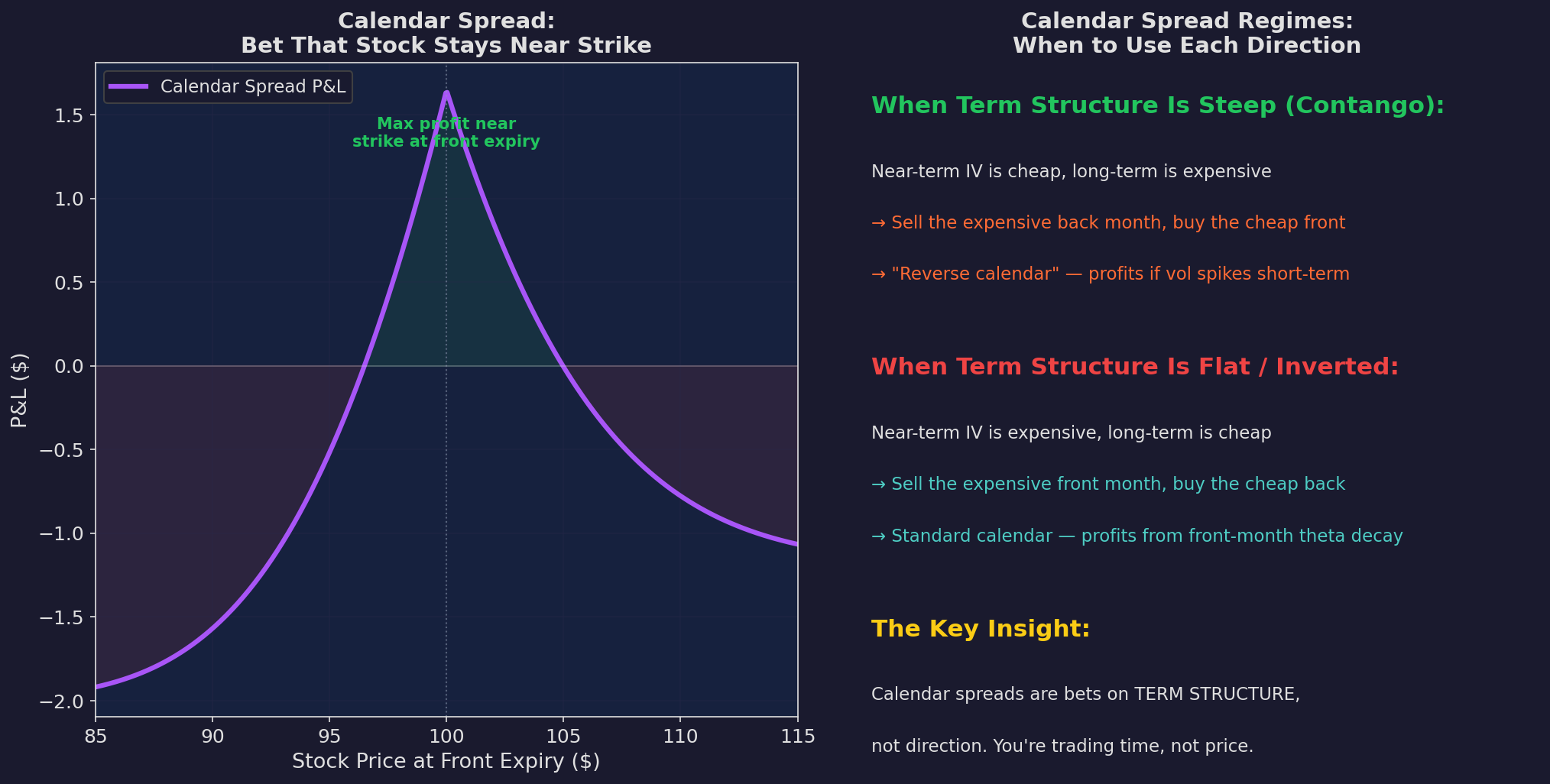
Left: the calendar spread payoff at front-month expiry. Maximum profit occurs near the strike price, where the back-month call retains maximum time value while the front-month call expires worthless. Right: regime-dependent calendar direction — sell expensive front-month vol when term structure is inverted, sell expensive back-month vol when term structure is steep.
The key insight: calendar spreads are not directional bets. They’re bets on the relative speed of time decay between two expirations. In a normal term structure, the front month decays faster (higher theta per day) — a standard calendar profits from this differential.
Calendar Trades for V6
V6 doesn’t currently trade calendars, but the term structure informs two decisions:
1. Expiry selection for the overlay (Part 4). When term structure is steep (contango), longer-dated options are expensive relative to near-term — buy shorter-dated protection. When inverted, shorter-dated options are overpriced — buy longer-dated protection.
2. Carry regime timing. VIX term structure inversion is one of the best carry crash indicators (Part 88). The calendar spread framework explains why — inversion means the market is paying more for near-term protection than long-term, which signals acute stress.
What the Surface Tells My V6
Here’s the practical extraction for a daily equity allocator:
Level (ATM IV / VIX): V6 already uses this via the VIX regime filter. High ATM vol = reduce allocation. This is the most important dimension and my V6 already captures it!
Skew (25-delta put-call IV spread): Extreme skew overshoots predict mean-reversion. For V6, this informs when to add back exposure after a selloff — if skew is extremely elevated but the selloff has paused, the market is pricing in too much further downside. This is a potential re-entry signal.
Term structure (VIX 1M/3M ratio): Inversion signals acute stress. V6 should treat term structure inversion as an independent warning alongside VIX level — you can have VIX at 22 with a normal term structure (fine) or VIX at 22 with an inverted structure (danger).
Convexity (wing pricing): Less relevant for V6’s daily allocation as it stands today (but that might change…) More relevant for the options overlay in Part 4, where we’ll use wing pricing to determine whether tail hedges are cheap or expensive.
The Honest Limitations
Vol surface trading is deep water. A few caveats:
1. Skew is expensive to trade. The bid-ask on OTM options is wide — 5-15% of the option’s value. A lot of the theoretical edge in skew trading gets eaten by spreads — unless you are doing this at scale and strategically, this is a significant consideration, especially for retail traders.
2. The surface moves. By the time you compute your z-scores and place the trade, the surface has shifted. Institutional vol desks have real-time feeds and sub-second execution. Retail has end-of-day data and limit orders.
3. Gamma risk. Short-dated skew trades have enormous gamma. A 1% move in the underlying can change the P&L of a weekly put spread by 50% of its maximum value. Position sizing must account for this.
4. Model risk. Everything above assumes Black-Scholes implied vols are the right metric. They’re not — they’re a convention. More sophisticated models (stochastic vol, local vol, rough vol) fit the surface better but require infrastructure that’s beyond most retail setups. It’s doable but you’ll need to invest significant time, energy, infrastructure and need a better command of the model.
For V6, the surface is primarily an input — a richer version of the VIX signal — rather than a tradeable opportunity in its own right. In Part 4, we’ll use surface information to design the options overlay, but we won’t try to trade the surface directly.
Up Next
Part 4: The V6 Options Overlay — Everything from Parts 90-92 converges into a specific overlay design. Tail hedge sizing using wing pricing, covered call income conditioned on skew, and the final assessment: is the added complexity worth the improved Sharpe?
Remember: Alpha is never guaranteed. And the backtest is a liar until proven otherwise.
These posts are about methodology, not recommendations. If you find errors in my math, let me know — I’ve built an entire series around discovering my own mistakes, so one more won’t hurt.
The material presented in Math & Markets is for informational purposes only. It does not constitute investment or financial advice.